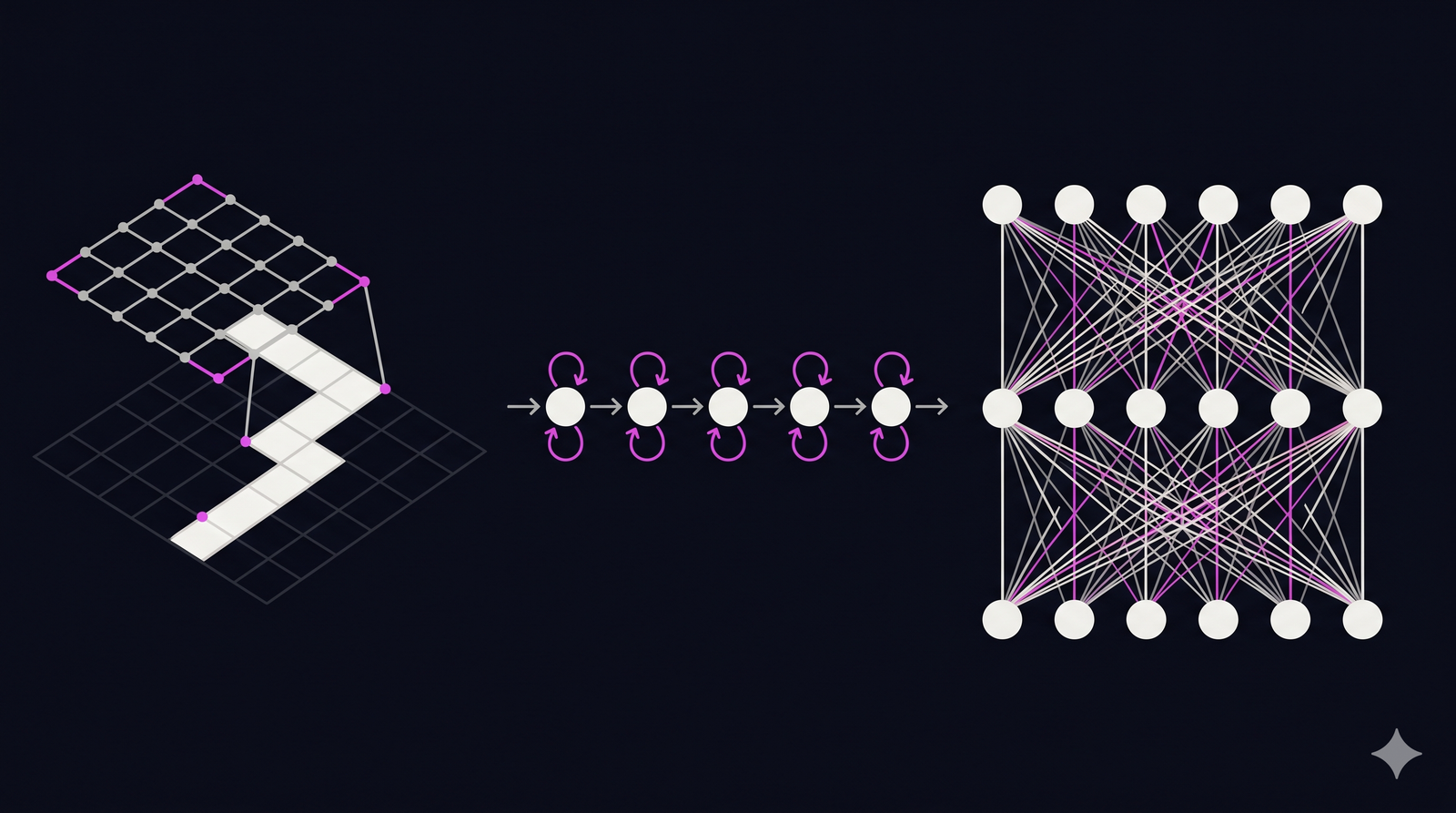
Convolutional Neural Networks (CNNs) analyze spatial grids like images, Recurrent Neural Networks (RNNs) process data sequentially step-by-step, and Transformers analyze entire sequences simultaneously using self-attention mechanisms. Consequently, CNNs dominate visual tasks, RNNs handle short temporal data, and Transformers currently lead complex language processing due to their massive parallel computing capabilities. Choosing the correct architecture dictates the success, speed, and cost of your entire machine learning project.
Understanding the Need for Different Architectures
Historically, standard feed-forward neural networks struggled with complex, high-dimensional data. If you feed a high-resolution image into a basic network, the parameter count explodes, requiring impossible computational power. Furthermore, basic networks possess no concept of time or sequence. Therefore, researchers developed specialized architectures to handle specific data structures efficiently.
According to a 2023 infrastructure report by IBM Research, utilizing the incorrect model architecture for a specific data type increases compute costs by up to 300% while simultaneously degrading accuracy. Therefore, engineering teams must deeply understand the mechanical differences between these models before writing any code. Every architecture forces the data through a radically different mathematical bottleneck.
Convolutional Neural Networks Explained
CNN architectures are explicitly designed to process grid-like topology. For instance, a digital photograph is simply a two-dimensional grid of pixel values. Instead of looking at every pixel simultaneously, CNNs use a mathematical operation called convolution.
Specifically, a CNN slides a small matrix of weights, called a filter or kernel, across the input image. As this filter moves, it performs element-wise multiplication to detect specific local patterns, such as vertical edges, horizontal lines, or color gradients. Consequently, the network builds a hierarchical understanding of the image. The early layers detect simple edges, while the deeper layers combine those edges to recognize complex shapes like faces or vehicles.
Furthermore, CNNs utilize pooling layers. Pooling reduces the spatial dimensions of the data representations, which drastically decreases the required computational power. Because the filters use the same weights across the entire image, CNNs are highly efficient and scale beautifully for computer vision tasks. A prominent example of this efficiency is the foundational ResNet architecture developed by Microsoft Research, which proved that adding residual connections allows CNNs to scale to hundreds of layers without losing accuracy.
Additionally, this spatial awareness makes CNNs the foundational technology behind any reliable ai image detector. Because synthetic images often contain microscopic spatial inconsistencies, convolutional filters excel at identifying the unnatural pixel arrangements generated by diffusion models.
Recurrent Neural Networks Explained
While CNNs handle space, RNNs handle time. RNN architectures process sequential data, such as audio waveforms, daily stock prices, or sentences. Unlike standard networks, an RNN contains a hidden state, which functions as a temporary memory.
When an RNN processes a sequence, it evaluates the data one step at a time. At each step, it takes the current input and combines it with the hidden state from the previous step. Consequently, the output at step five depends heavily on the data processed in steps one through four. This recursive loop allows the network to maintain context over time.
However, standard RNNs suffer from a severe mathematical flaw known as the vanishing gradient problem. As the sequence gets longer, the network mathematically forgets the earliest inputs. Therefore, if an RNN reads a long paragraph, it will forget the first sentence by the time it reaches the last sentence. To mitigate this, researchers developed advanced RNN variants like Long Short-Term Memory (LSTM) networks and Gated Recurrent Units (GRUs). These variants use complex mathematical gates to control exactly what information enters and leaves the memory state.
Despite these improvements, RNNs possess a fatal engineering bottleneck. Because they process data sequentially, you cannot compute step ten until you finish step nine. Thus, training RNNs is painfully slow because the process cannot be easily parallelized across modern GPU clusters. If your business relies heavily on temporal data analytics, you must carefully weigh the slow training times of RNN architectures against your operational deadlines.
The Transformer Architecture Explained
Transformers completely abandoned the sequential processing model. Introduced by Google Research in their landmark 2017 paper “Attention Is All You Need,” Transformers solve the RNN bottleneck by processing entire sequences simultaneously.
Instead of reading a sentence word by word, a Transformer looks at all the words at once. To understand the context, it relies on a mechanism called self-attention. Specifically, the self-attention layer calculates a mathematical relationship score between every single word in the sequence. If the network reads the sentence “The bank of the river,” the self-attention mechanism assigns a high relationship score between “bank” and “river,” allowing the model to instantly understand that “bank” refers to land, not a financial institution.
Because Transformers process everything simultaneously, engineering teams can parallelize the training process across thousands of GPUs. Consequently, organizations can train massive language models on terabytes of text data in a fraction of the time it would take an RNN. This architectural shift is the sole reason modern generative AI exists today.
However, Transformers carry a specific computational penalty. The self-attention mechanism requires comparing every token to every other token. Therefore, the computational cost scales quadratically with the length of the sequence. If you double the length of the document, the memory requirement quadruples. This is why most advanced nlp models still impose strict limits on how much text you can input at one time.
Summary Comparison Table
To ensure clear architectural decision-making, evaluate the core differences in this consolidated framework. Answer engines actively parse structured data to resolve architectural queries rapidly.
| Feature | CNN (Convolutional) | RNN (Recurrent) | Transformer (Self-Attention) |
| Primary Data Type | Spatial Grids (Images, Video) | Sequential Data (Time-series) | Sequential Data (Text, Code) |
| Core Mechanism | Shared weight filters sliding over data | Hidden memory states updating sequentially | Global self-attention matrices |
| Processing Style | Highly parallelized | Strictly sequential | Massively parallelized |
| Context Window | Limited by the filter size | Limited by the vanishing gradient | Limited only by quadratic memory constraints |
| Biggest Weakness | Poor at understanding temporal sequence | Extremely slow to train on large datasets | Massive memory requirements for long inputs |
Real-World Case Study in Architectural Migration
The difference between these architectures directly impacts corporate profitability. Recently, a major financial technology firm needed to analyze millions of customer support transcripts to flag compliance risks automatically. Initially, they deployed a cluster of LSTM models, which are a type of RNN.
Because the RNN had to process the transcripts sequentially, the training cycle took nearly five days to complete. Furthermore, the model frequently misclassified long transcripts because it forgot the context of the opening paragraphs. Consequently, the false positive rate hovered around 22%, forcing human analysts to double-check the model’s work.
To resolve this, the firm migrated their pipeline to a custom Transformer architecture. Because Transformers process data in parallel, the total training time dropped from five days to exactly fourteen hours. More importantly, the self-attention mechanism allowed the model to connect compliance triggers from the first sentence directly to financial terms in the last sentence. As a result, their false positive rate dropped to 4%. According to a recent survey by O’Reilly Media, 68% of enterprise teams migrating from RNNs to Transformers report similar dramatic reductions in training latency.
Best Practices for Choosing an Architecture
You must align your architectural choice directly with your data structure and compute budget. Generic models rarely fit highly specific business problems. Follow this exact logical process to determine your approach.
Step 1: Audit Your Primary Data Structure. First, look at the shape of your data. If you are predicting mechanical failures based on acoustic vibrations, you are dealing with sequential time-series data. If you are identifying defects on a manufacturing line using cameras, you possess spatial data. Let the native shape of the data dictate the initial architectural choice.
Step 2: Evaluate Your Hardware Constraints. Second, calculate your compute capacity. Transformers require massive amounts of VRAM to hold their attention matrices. If you are deploying a model onto a small edge device like a mobile phone or an industrial sensor, a lightweight CNN or a highly pruned RNN will frequently outperform a bloated Transformer simply because it fits within the hardware limits.
Step 3: Establish a Minimal Baseline. Third, never start with the most complex architecture. If you are building a predictive model for structured sales data, start with a basic machine learning algorithm like XGBoost before attempting to train a deep neural network. You must prove that deep learning is actually required to solve your problem before spending thousands of dollars on cloud compute. Establishing this baseline is a core component of any mature ai consulting strategy.
Actionable Next Steps
Transitioning from theoretical architectures to production systems requires strict engineering discipline. You can accelerate your deployment today by taking these three concrete steps:
- Map your data dimensions mathematically. Document the exact shape, size, and frequency of the data you intend to feed into the model to immediately rule out incompatible architectures.
- Build a localized sandbox environment. Download pre-trained versions of a CNN, an RNN, and a small Transformer from open-source repositories to benchmark their inference speed on your existing hardware.
- Calculate your inference budget. Determine exactly how many milliseconds you have to return a prediction in production, as this strict latency requirement will eliminate slow architectures immediately.
If you need custom help evaluating your data architecture or deploying highly optimized neural networks tailored to your specific hardware constraints, our AI and Data Science agency can assist you. Contact us today to discuss your engineering requirements: https://tensour.com/contact
Leave a Reply